Further Study
So far, we have mostly discussed supervised learning. In supervised learning, the model is trained on a labeled dataset. This means that each input comes with the correct answer. The goal is to learn a rule that works not only on the training examples, but also on new, unseen examples.
Pros:
High accuracy when enough labeled data is available.
Predictable performance and easier to evaluate.
Well-supported with mature libraries.
Cons:
Requires large, clean labeled datasets, which can be expensive or time-consuming to produce.
May overfit if there is not enough data or if the model is too complex.
Unsupervised models
Unsupervised learning works with unlabeled data. Here, the model is not told the correct answer. Instead, it tries to discover hidden patterns, groups, or useful representations inside the data. Rather than covering this in the limited time of this course, we have an exercise on unsupervised learning for you to learn on your own.
For example, if we give a model many customer profiles without labels, it may discover groups of customers with similar purchasing habits. In physics, unsupervised methods can also be useful for anomaly detection, dimensionality reduction, compression, and representation learning.
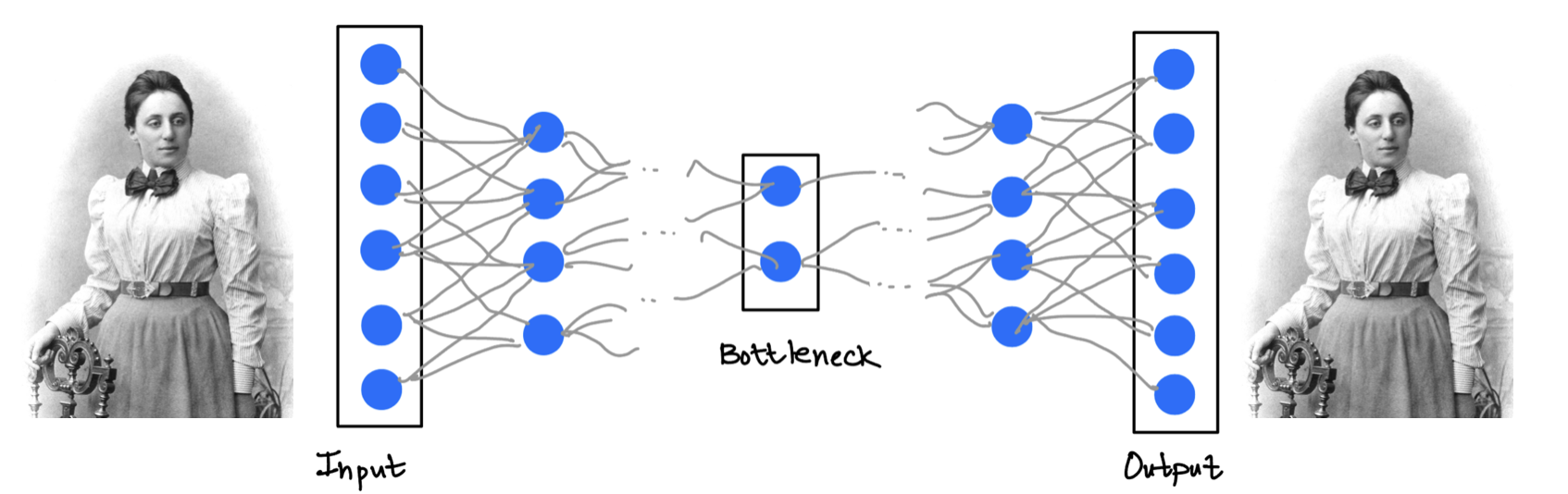
One important example is an autoencoder. An autoencoder tries to compress the input into a smaller hidden representation and then reconstruct the original input from that representation. If the reconstruction works well, the hidden representation has captured something useful about the data.
Example: Autoencoder
Pros:
Works without labeled data.
Helps with data exploration, dimensionality reduction, compression, and pattern discovery.
Cons:
Harder to evaluate, because there is no obvious ground truth label.
May discover patterns that are mathematically real but physically or practically unimportant.
Often requires care in interpreting what the model has learned.
Boltzmann machines: when statistical mechanics learns from data
Another important unsupervised model comes almost directly from statistical mechanics.
A Boltzmann machine is a network of stochastic binary units. Each unit can be either on or off, rather like an Ising spin that can point in one of two directions.
Some units are called visible units because they represent the data that we observe. Other units are called hidden units, which are allowed to learn patterns and correlations that were not explicitly given to the model.
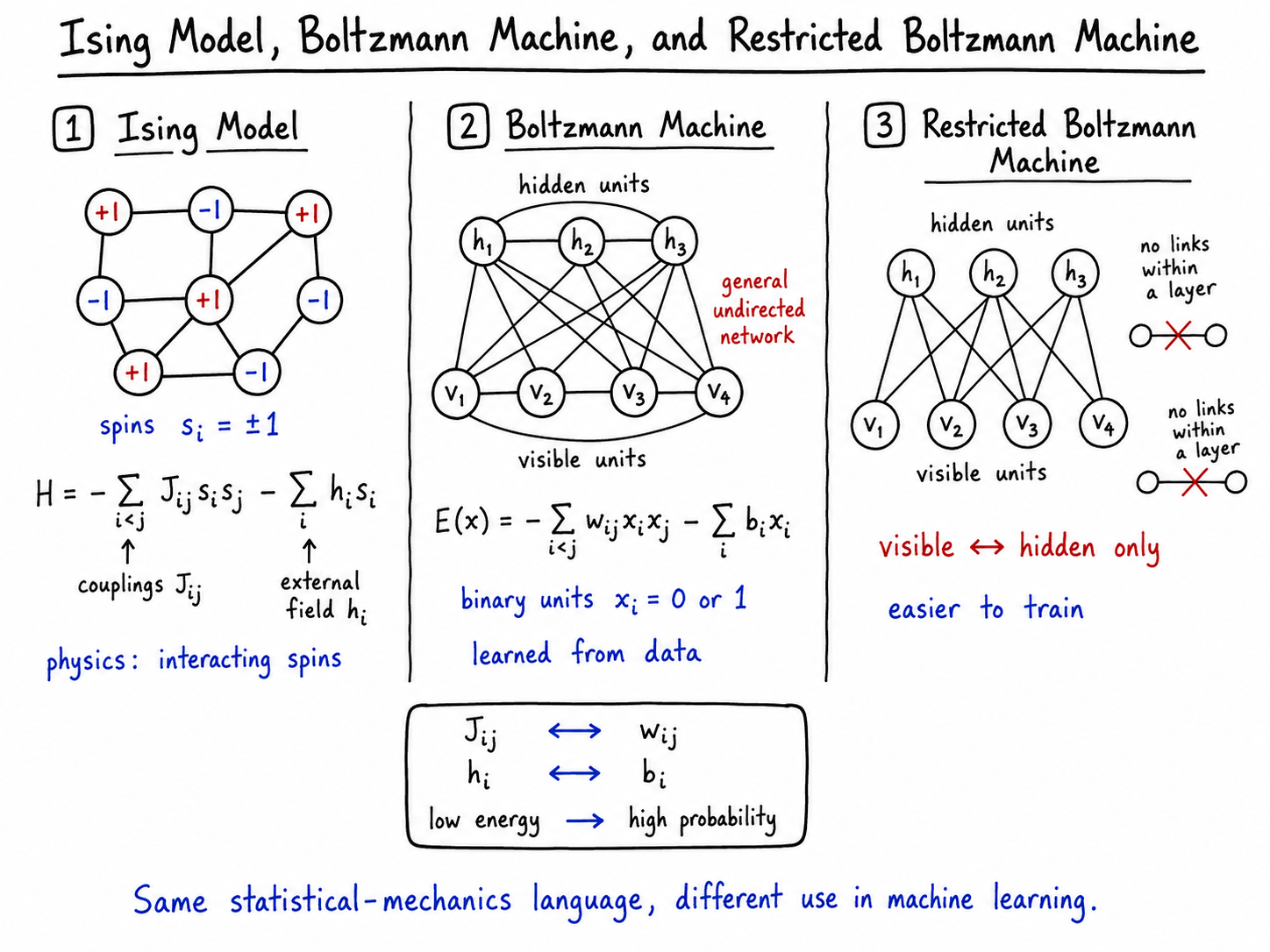
The Ising model and the Boltzmann machine use the same basic language: configurations, interactions, energies, and probabilities.
From energy to probability
Suppose each binary unit has a state
A Boltzmann machine assigns an energy to every possible configuration:
Here:
is the interaction between units and ;
is the bias acting on unit ;
represents the complete configuration of the network.
The energy is converted into a probability through the Boltzmann distribution,
where
is the partition function.
In most machine-learning discussions, the temperature is set to , or absorbed into the weights and biases.
The connection with the Ising model
The Hamiltonian of an Ising model can be written as
where
Compare this with the energy of the Boltzmann machine:
The correspondence is almost immediate:
| Ising model | Boltzmann machine |
|---|---|
| spin | binary unit |
| coupling | learnable weight |
| external field | learnable bias |
| Hamiltonian | model energy |
| thermal configuration | data configuration |
| Boltzmann probability | model probability |
The two binary conventions are related by
What is the machine trying to learn?
A standard Boltzmann machine is mainly an unsupervised generative model.
It tries to learn the probability distribution
of the observed data.
During training, the weights are adjusted so that
configurations resembling the data   → lower energy → higher probability

unrealistic configurations           → higher energy → lower probability
Hidden units allow the model to represent correlations that may not be obvious from the visible variables alone.
For the mathematically curious students
The learning rule for a weight has the schematic form
The first term measures how strongly units and are correlated when the network is shown the data.
The second term measures the correlation produced by the model’s own probability distribution.
Training therefore asks the model ensemble to reproduce the correlations observed in the data ensemble.
A physicist may recognize the spirit immediately: we are comparing expectation values in two statistical ensembles.
Visible and hidden units
Let us separate the network into
visible units , which represent the observed data;
hidden units , which learn additional internal structure.
The model assigns a joint probability
Since the hidden units are not directly observed, the probability of a visible configuration is obtained by summing over every possible hidden configuration:
Because the model learns a full probability distribution, it can in principle generate new configurations resembling the training data.
Boltzmann machine versus restricted Boltzmann machine
In a general Boltzmann machine, many pairs of units may be connected. This makes the model expressive, but it also makes exact training and sampling difficult.
A Restricted Boltzmann Machine, or RBM, imposes a simpler structure:
visible units connect to hidden units;
visible units do not connect directly to other visible units;
hidden units do not connect directly to other hidden units.
visible layer ↔ hidden layerThis restriction makes the conditional probabilities much easier to calculate.
Is a Boltzmann machine supervised or unsupervised?
A standard Boltzmann machine is primarily an unsupervised generative model.
It learns
the probability distribution of the data, without requiring a class label for every example.
However, labels can also be included among the visible variables. The model may then learn
and classification can be performed using
So the clean statement is:
A conventional Boltzmann machine is unsupervised, but related versions can also be adapted for supervised classification.
Reinforcement Learning
Reinforcement learning is different from both supervised and unsupervised learning. Here, the model is usually called an agent. The agent interacts with an environment, takes actions, and receives rewards or penalties.
The goal is not simply to predict a label. The goal is to learn a good strategy.
A typical reinforcement learning loop looks like this:
For example, a robot learning to walk, a program learning to play chess, or an algorithm learning how to control a system can all be thought of in this framework.
Pros:
Very useful for sequential decision-making and control tasks.
Learns from interaction rather than from a fixed labeled dataset.
Can discover strategies that are difficult to write down by hand.
Cons:
Often slow and computationally expensive.
May require a lot of exploration or simulation before learning effectively.
Rewards must be designed carefully, otherwise the agent may learn the wrong behavior.
Trending Topics in ML
Machine learning moves quickly. New model names appear every week, and sometimes an old idea returns wearing a much larger neural network and a much more expensive coat.
This section is therefore not a list of everything fashionable at this moment. Instead, it is a short guide to a few ideas that you are likely to encounter when reading modern ML papers, preparing scientific datasets, or working with AI tools.
1. From CSV to Parquet and Arrow
A table can be stored in many different ways. The familiar CSV format writes values as plain text. It is easy to open and inspect, but it has several limitations as you have seen before from the work we did with the decision tree section:
the data types are not stored very carefully;
files can become large;
reading one or two columns may still require scanning much of the file;
nested or complicated data are awkward to represent.
Parquet is a compressed, column-oriented file format. Instead of organizing the file mainly row by row, it keeps values from the same column together. This is useful when we have a large table but need only a few observables.
For example, an event table may contain
event_id, jet_pt, jet_eta, jet_mass, MET, number_of_tracks, label, ...If our analysis needs only jet_pt and jet_mass, a columnar format can avoid reading every other column.
Apache Arrow is closely related, but it is useful to keep the distinction clear:
Parquet mainly describes how columnar data are stored in a file.
Arrow mainly describes how columnar data can be represented efficiently in memory and exchanged between programs.
A typical command would look like
small_table = pd.read_parquet(
    "events.parquet",
    columns=["jet_pt", "jet_mass"],
)
Here the columns=... argument states explicitly that the analysis does not need the entire table. This command is shown only as an illustration because reading Parquet files requires an additional engine such as pyarrow, which we do not load inside the browser.
The example below does not write a real Parquet file because that would require an additional Parquet engine. It demonstrates the more important idea: selecting only the columns required by the analysis, by simply mimicking what parquet format does with the data. You will encounter this during your exercises.
import numpy as np
import pandas as pd

rng = np.random.default_rng(42)

events = pd.DataFrame({
    "event_id": np.arange(1, 9),
    "jet_pt": rng.uniform(30, 500, size=8),
    "jet_eta": rng.normal(0, 1.2, size=8),
    "jet_mass": rng.uniform(5, 180, size=8),
    "MET": rng.uniform(0, 250, size=8),
    "number_of_tracks": rng.integers(5, 80, size=8),
    "label": rng.choice(["q", "g", "W", "Z", "t"], size=8),
})

print("The complete event table contains:")
print(list(events.columns))

columns_needed_for_this_analysis = events[["jet_pt", "jet_mass"]]

print("\nFor this analysis we read only:")
columns_needed_for_this_analysis.round(2)
The complete event table contains:
['event_id', 'jet_pt', 'jet_eta', 'jet_mass', 'MET', 'number_of_tracks', 'label']

For this analysis we read only:
2. What does an “ML-ready dataset” mean?
An ML-ready dataset is not a special file extension. A Parquet file can still contain terrible data, and a humble CSV file can contain an excellent dataset.
“ML-ready” means that the dataset has been prepared well enough for a particular machine-learning task.
At minimum, we should know:
What does each row represent?
What does each feature mean, and what units does it use?
What is the target or label?
Are any values missing, impossible, duplicated, or corrupted?
Are the classes strongly imbalanced?
How were the training, validation, and test samples defined?
Could two entries from the same physical event appear in different splits?
Was any information from the test sample used during preprocessing?
Where did the data come from, and which processing steps were applied?
Let us inspect a deliberately messy toy dataset.
messy_events = pd.DataFrame({
    "event_id": [101, 102, 103, 103, 105],
    "jet_pt_GeV": [120.0, 85.0, np.nan, 210.0, -15.0],
    "jet_mass_GeV": [80.4, 12.5, 91.2, 91.2, 170.0],
    "label": ["W", "q", "Z", "Z", None],
})

print("Data types:")
print(messy_events.dtypes)

print("\nMissing values:")
print(messy_events.isna().sum())

print("\nNumber of duplicated rows:")
print(messy_events.duplicated().sum())

print("\nNumber of repeated event IDs:")
print(messy_events["event_id"].duplicated().sum())

print("\nClass counts:")
print(messy_events["label"].value_counts(dropna=False))

print("\nThe suspicious negative transverse momentum is:")
messy_events[messy_events["jet_pt_GeV"] < 0]
Data types:
event_id          int64
jet_pt_GeV      float64
jet_mass_GeV    float64
label            object
dtype: object

Missing values:
event_id        0
jet_pt_GeV      1
jet_mass_GeV    0
label           1
dtype: int64

Number of duplicated rows:
0

Number of repeated event IDs:
1

Class counts:
label
Z       2
W       1
q       1
None    1
Name: count, dtype: int64

The suspicious negative transverse momentum is:
The checks above do not magically repair the dataset. They tell us where to begin asking questions.
For example:
Is the repeated
event_ida true duplicate, or does one event contain several jets?Why is one transverse momentum negative?
Is the missing label recoverable, or should the event be removed?
Are the units really GeV everywhere?
This is why data preparation is not merely the boring step before machine learning. In many scientific projects, it is the place where most mistakes are either prevented or quietly introduced.
3. Dataset cards, schemas, provenance, and versioning
Once a dataset is prepared, another person should be able to understand what it contains without reading the mind of its creator.
A few useful ideas are:
A schema records the feature names, data types, shapes, and often units.
Provenance records where the data came from and which processing steps produced the current form.
Versioning distinguishes one release of the dataset from another.
A dataset card gives a human-readable summary of the dataset, its intended use, and its known limitations.
A minimal scientific dataset card might answer:
What is this dataset?
Who created it?
How was it generated or collected?
Which features and labels are included?
How are the train, validation, and test splits defined?
What should the dataset be used for?
What should it not be used for?
What limitations are already known?Below is a tiny machine-readable dataset description. In a real project, the same information could be stored in YAML, JSON, or a dedicated metadata system.
import json

dataset_card = {
    "name": "Toy Jet Dataset",
    "version": "1.0.0",
    "task": "five-class jet classification",
    "features": {
        "jet_pt": "transverse momentum in GeV",
        "jet_eta": "pseudorapidity",
        "jet_mass": "jet mass in GeV",
    },
    "label": {
        "name": "jet_type",
        "classes": ["q", "g", "W", "Z", "t"],
    },
    "splits": {
        "train": "70%",
        "validation": "15%",
        "test": "15%",
    },
    "provenance": "Toy data generated for this notebook",
    "known_limitations": [
        "not detector data",
        "no pileup",
        "not suitable for a physics result",
    ],
}

print(json.dumps(dataset_card, indent=2))
{
  "name": "Toy Jet Dataset",
  "version": "1.0.0",
  "task": "five-class jet classification",
  "features": {
    "jet_pt": "transverse momentum in GeV",
    "jet_eta": "pseudorapidity",
    "jet_mass": "jet mass in GeV"
  },
  "label": {
    "name": "jet_type",
    "classes": [
      "q",
      "g",
      "W",
      "Z",
      "t"
    ]
  },
  "splits": {
    "train": "70%",
    "validation": "15%",
    "test": "15%"
  },
  "provenance": "Toy data generated for this notebook",
  "known_limitations": [
    "not detector data",
    "no pileup",
    "not suitable for a physics result"
  ]
}
4. Foundation models, pretraining, and transfer learning
Earlier in this course, we usually trained a model for one clearly defined task. A foundation model begins from a broader idea:
train once on a large and varied collection of data
                         ↓
learn a reusable representation
                         ↓
adapt the model to many smaller downstream tasks
The first stage is called pretraining. The later adaptation may happen through:
fine-tuning, where some or all model parameters are updated;
using the pretrained network as a fixed feature extractor;
adding a small task-specific head;
prompting or providing examples in the input context.
This is a more ambitious version of transfer learning: knowledge acquired from one broad training process is reused elsewhere.
A familiar example is an image model that first learns general visual structure and is later adapted to classify a specialized set of detector images. In language models, broad pretraining can later be adapted to summarization, coding, question answering, or scientific writing.
A multimodal model extends the idea by learning from more than one kind of input—for example text and images, or detector readouts together with written metadata. The central question is whether the model can learn a useful common representation across those different forms of information.
Large pretraining is therefore not automatically the best solution to every scientific problem. Sometimes a smaller model with the right physical variables and the right inductive bias is the wiser machine.
5. Embeddings, vector search, and RAG
An embedding, as you have seen, converts an object into a vector of numbers:
The object could be a sentence, an image, a particle collision event, a molecule, or an entire document. The hope is that objects with similar meaning or structure end up close to one another in the embedding space.
Once objects are represented by vectors, we can search for nearby objects using a similarity measure such as the cosine similarity,
The following vectors are hand-made only for illustration. A real embedding model would learn them from data.
abstract_vectors = {
    "jet classification": np.array([0.95, 0.80, 0.10]),
    "detector monitoring": np.array([0.70, 0.95, 0.15]),
    "black-hole thermodynamics": np.array([0.05, 0.10, 0.98]),
    "particle-flow reconstruction": np.array([0.85, 0.75, 0.20]),
}

query = np.array([0.90, 0.85, 0.12]) # This is the "word vector" that we want to compare to the abstract vectors.

def cosine_similarity(a, b):
    return np.dot(a, b) / (
        np.linalg.norm(a) * np.linalg.norm(b)
    )

similarities = {
    name: cosine_similarity(query, vector)
    for name, vector in abstract_vectors.items()
}

pd.Series(similarities, name="cosine similarity").sort_values(
    ascending=False
).round(3)
jet classification              0.998
particle-flow reconstruction    0.996
detector monitoring             0.984
black-hole thermodynamics       0.202
Name: cosine similarity, dtype: float64
A vector database is a system designed to store many such vectors and efficiently retrieve nearby ones.
This leads naturally to retrieval-augmented generation, usually called RAG:
question
   ↓
retrieve relevant documents or passages
   ↓
place the retrieved material in the model's context
   ↓
generate an answer using that additional information
The important point is that retrieval and generation are different jobs.
The model does not need to memorize every paper forever. It can first retrieve useful external material and then work with what was found.
6. AI agents, tool calling, and MCP
A language model produces text or structured output. An agentic system places that model inside a loop where it may also choose and use external tools.
A simplified agent loop is
understand the request
        ↓
decide whether a tool is needed
        ↓
choose a tool and prepare its inputs
        ↓
run the tool
        ↓
inspect the result
        ↓
answer, or take another step
Tools may include:
a calculator;
a search engine;
a database;
a calendar;
a Python function;
a ROOT-file reader;
a detector-monitoring service;
or an event generator.
The Model Context Protocol, or MCP, is an open standard for connecting AI applications to external systems through a common interface.
Three useful MCP ideas are:
resources provide contextual data, such as files or database records;
tools perform actions or computations;
prompts provide reusable instruction templates.
The following is not a real MCP server. It is a tiny analogy showing how a model or program may discover a tool by name and call it with structured arguments.
import json
import numpy as np


# Functions that our simple agent can use
def mean(values):
    return sum(values) / len(values)


def invariant_mass(energy, px, py, pz):
    """Calculate invariant mass from the four-momentum."""
    mass_squared = energy**2 - px**2 - py**2 - pz**2

    # Protect against tiny negative values from numerical precision
    return np.sqrt(max(mass_squared, 0.0))


# The tool registry connects each tool name to a Python function
tools = {
    "mean": mean,
    "invariant_mass": invariant_mass,
}


# A structured request specifying the tool and its arguments
tool_request = {
    "tool": "invariant_mass",
    "arguments": {
        "energy": 125.0,
        "px": 30.0,
        "py": 20.0,
        "pz": 90.0,
    },
}


def call_tool(request):
    """Find the requested tool and call it with the supplied arguments."""
    tool_name = request["tool"]
    arguments = request["arguments"]

    if tool_name not in tools:
        raise ValueError(f"Unknown tool: {tool_name}")

    # **arguments passes the dictionary entries as named arguments
    return tools[tool_name](**arguments)


result = call_tool(tool_request)

print("Structured request:")
print(json.dumps(tool_request, indent=2))
print(f"\nTool result: {result:.3f}")
Structured request:
{
"tool": "invariant_mass",
"arguments": {
"energy": 125.0,
"px": 30.0,
"py": 20.0,
"pz": 90.0
}
}
Tool result: 78.899
7. Generative models and synthetic data
A discriminative model learns to predict something about the data, for example
A generative model tries to learn enough about the data distribution to create new samples that resemble the original data.
Important families include:
variational autoencoders;
generative adversarial networks;
normalizing flows;
diffusion models;
flow-matching models.
In scientific applications, generative models can be used for fast simulation, detector-response modelling, data augmentation, inverse problems, and probabilistic reconstruction. My future plans include writing a course on generative models, keep an eye open for that in this course page or be in touch with me.
8. Reproducible ML and lightweight MLOps
The word MLOps refers broadly to the practices used to build, track, test, deploy, and maintain machine-learning systems.
For this course, we need only the scientific core of the idea:
record the random seed;
record the dataset version;
save the feature definitions and preprocessing;
save the train, validation, and test split;
record the model architecture and hyperparameters;
record the software versions;
save the trained parameters;
record which run produced each figure or number.
This is not bureaucracy added after the science. It is how we remember what the science actually was.
A small experiment record may look like this:
import hashlib
import sys

dataset_fingerprint = hashlib.sha256(
    pd.util.hash_pandas_object(events, index=True)
    .values
    .tobytes()
).hexdigest()[:12]

experiment_record = {
    "experiment_name": "toy_jet_classifier",
    "dataset_version": "1.0.0",
    "dataset_fingerprint": dataset_fingerprint,
    "random_seed": 42,
    "features": ["jet_pt", "jet_eta", "jet_mass"],
    "split": {
        "train": 0.70,
        "validation": 0.15,
        "test": 0.15,
    },
    "learning_rate": 1e-3,
    "batch_size": 64,
    "python_version": sys.version.split()[0],
    "numpy_version": np.__version__,
    "pandas_version": pd.__version__,
}

print(json.dumps(experiment_record, indent=2))
9. Trustworthy ML: leakage, calibration, bias, and unfamiliar data
A model can have impressive accuracy and still be scientifically unsafe.
Four questions are especially useful.
Data leakage
Did information about the answer accidentally enter the inputs or preprocessing?
Examples include:
normalizing with the full dataset before splitting;
placing related events in both training and test samples;
including a feature constructed using truth information;
repeatedly tuning on the final test set.
Calibration
If a model says “90% confidence” many times, is it correct roughly 90% of those times?
Accuracy asks whether the winning class is correct. Calibration asks whether the reported probabilities deserve to be interpreted as probabilities.
Out-of-distribution data
What happens when the new data differ from the training sample?
A model trained on one detector condition, generator tune, pileup range, or phase-space region may behave unpredictably elsewhere.
Bias and uneven performance
Does the average score hide a region or class where the model performs badly?
10. Scientific machine learning
Scientific machine learning asks how data-driven methods and scientific knowledge can work together.
There are several directions.
ML for science
Use machine learning as a tool for:
classification and regression;
anomaly detection;
surrogate simulation;
parameter inference;
reconstruction;
experimental control.
Physics inside ML
Build known structure into the model:
symmetries and equivariance;
conservation laws;
dimensional constraints;
causal or geometric structure;
differential equations;
graph structure and locality;
known numerical solvers or differentiable simulators.
ML for discovering physics
Use flexible models to identify patterns, effective descriptions, latent variables, or candidate equations that were not supplied in advance.
Other active directions include graph neural networks for relational data, neural operators that learn maps between functions, and scientific foundation models pretrained across large collections of simulations, measurements, structures, or scientific text. Their ambition is similar to that of other foundation models: learn a reusable representation first, and adapt it to many later scientific tasks.
One simple idea used in physics-informed learning is to penalize a model when it violates a known equation. NOTE: This will just make things approximate, incorporating exact symmetries or rules needs much more precision or thoughts.
A physics-informed neural network (PINN) can use a related residual as one part of its loss function. The network is then asked not only to fit the available data, but also to remain compatible with known physics.
Final takeaway
The topics in this section may look unrelated:
Parquet and Arrow concern how data are stored and moved.
ML-ready datasets and dataset cards concern whether data can be understood and trusted.
Foundation models and embeddings concern reusable representations.
RAG, agents, and MCP concern how models obtain context and use tools.
Generative models concern learning and sampling distributions.
MLOps and reproducibility concern remembering exactly what was done.
Trustworthy ML concerns knowing when a model may fail.
Scientific ML concerns combining learning with structure already known from science.
But they are connected by one larger lesson:
For physicists, the future is probably not physics or machine learning.
It is learning where known physics should be built into the system, where data should be allowed to speak, and where neither should be trusted without a careful cross-check.