Practical Example: ML for HEP

You are already familiar with the scale of data that physicists have to handle. Even checking whether a large experiment is operating properly may require looking through thousands of histograms and detector quantities. Machine Learning can help us reduce some of this human effort, search large datasets quickly, and identify patterns that may otherwise remain hidden.

One should nevertheless remember that the goal of ML in physics is not to replace the physics simulation or physical reasoning. The goal is to aid them. For example, automating parts of Data Quality Monitoring (DQM) could reduce the burden on detector shifters, while the final interpretation must still remain grounded in physics.

The goal of particle physics is to understand the nature, towards that we can use ML in several possible places

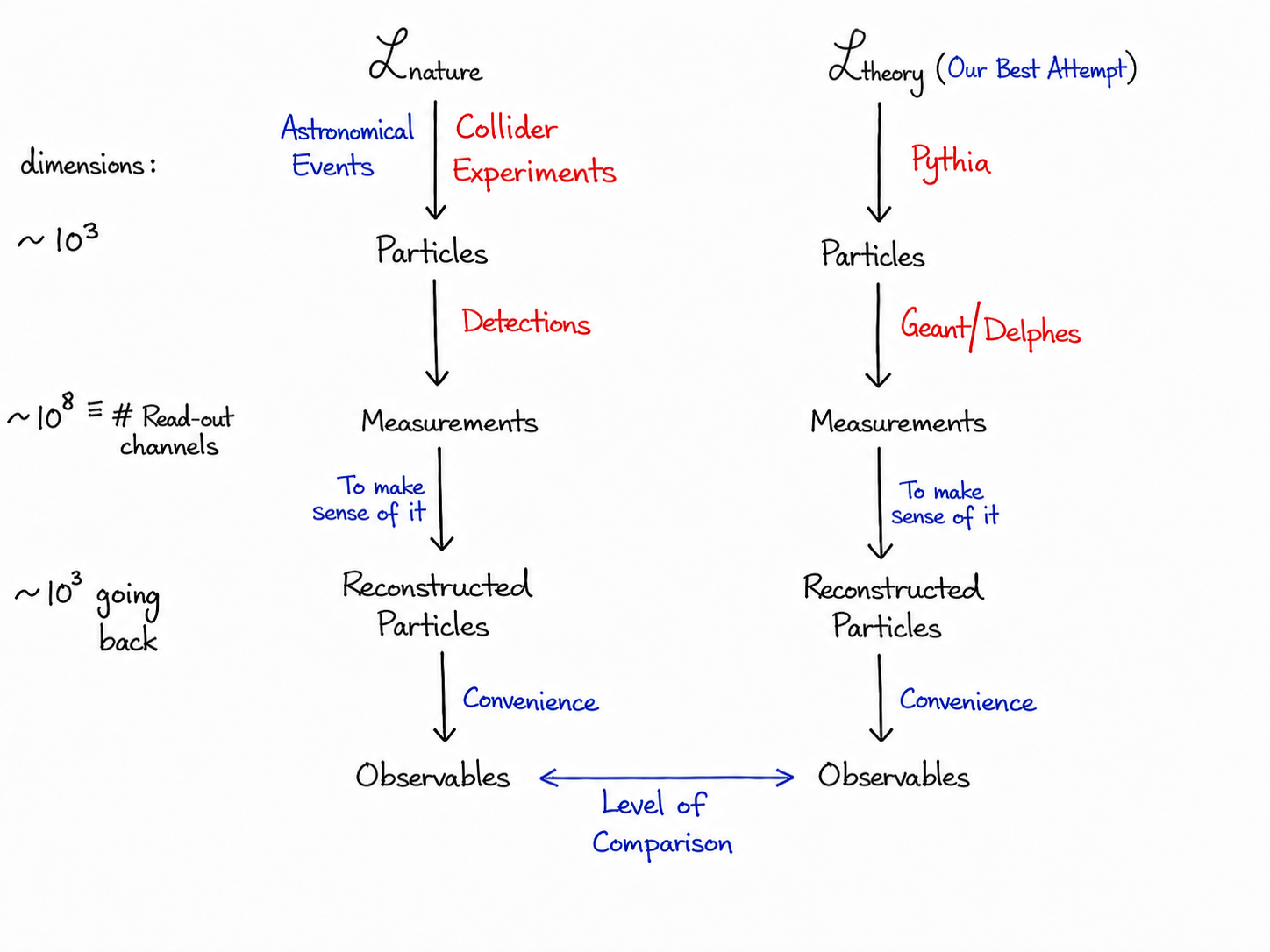
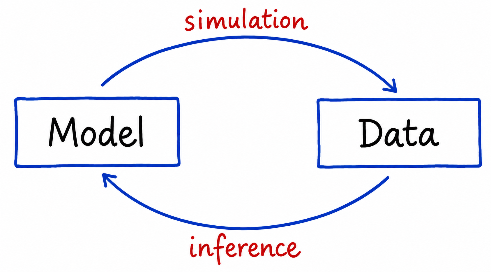
• This also brings us toward an inference-based approach to understanding nature, or in other words, the Standard Model.

Jet classification with PyTorch¶

We will now work through a compact but complete example of a deep-learning analysis in High-Energy Physics. The aim is not merely to run a finished neural network. We will prepare the data, construct the model, train it, inspect its failures, and ask whether the final result makes physical sense.

The Task¶

We will use the hls4ml Jet High-Level Features dataset, stored as hls4ml_HLF.arff when available locally. Our goal is to classify jets from proton-proton collisions into five categories:

• g: gluon jets, represented by label 0;

• q: quark jets, represented by label 1;

• w: hadronically decaying $W$ bosons, represented by label 2;

• z: hadronically decaying $Z$ bosons, represented by label 3;

• t: hadronically decaying top quarks, represented by label 4.

Each jet is represented by 16 high-level features describing properties such as its shape, mass, energy distribution, and constituent multiplicity.

The full dataset contains many events. To keep this suitable for a short course, we begin with a smaller random sample. Once the full pipeline works, you can always scale it up.

Imports and hardware check¶

First, we import the packages that will be needed throughout the notebook. We also ask PyTorch whether an accelerator is available:

• CUDA is used for supported NVIDIA GPUs;

• MPS is used for supported Apple Silicon GPUs;

• otherwise, the notebook falls back to the CPU.

The same code can therefore run on several types of machines.

❓ Exercise¶

Q20: What is nn vs F? Why does PyTorch separate them? (Hint: Think about stateful object-oriented layers vs stateless mathematical functions).

Q21: Why do we use DataLoader instead of just feeding the entire dataset into the model at once? What memory and optimization benefits does it provide?

Q22: What is CUDA or MPS? Why is GPU training so much faster than CPU training for deep learning?

Load and Prepare the Dataset¶

We now prepare the dataset step by step before giving it to the neural network.

1. Load the ARFF file:
   ARFF stands for Attribute-Relation File Format. It is a text-based format commonly used in machine learning that stores both the description of the dataset—such as feature names and data types—and the actual data values.

2. Decode the class labels:
   The labels may initially be stored as byte objects such as b'q' or b'g'. We decode them into ordinary Python strings such as 'q' and 'g', which are easier to inspect and work with.

3. Convert labels into numbers:
   A neural network cannot directly learn from text labels. We therefore map each jet class to an integer, for example,

   q → 0
   g → 1
   w → 2
   z → 3
   t → 4

   These integers tell PyTorch which class each event belongs to.

4. Take a random subset:
   The complete dataset is quite large. To make the first training exercise faster, we randomly select a smaller number of events. Because the sample is chosen randomly, it should still approximately represent the full dataset.

5. Split the data:
   We divide the selected events into a training set and a test set. The model learns from the training set, while the test set is kept aside to check how well the trained model performs on events it has not seen before.

6. Normalize the input features:
   Different jet observables can have very different numerical ranges. We use StandardScaler to transform each feature so that it has approximately zero mean and unit variance. This prevents features with large numerical values from dominating the training.

   Importantly, the scaler is fitted only on the training data and then applied to the test data. This avoids accidentally passing information from the test set into the training procedure.

7. Convert everything into PyTorch tensors:
   Finally, we convert the NumPy arrays into PyTorch tensors. The input features are stored as floating-point tensors, while the class labels are stored as integer tensors. These are the formats expected by the neural network and the classification loss function.

After these steps, the data are ready to be grouped into batches and passed through the neural network.

What information are we giving to the neural network?¶

Before training the neural network, let us first inspect the input features.

Each row of the dataset represents one jet, while each column contains a numerical description of some aspect of that jet. These numbers summarize questions such as:

• How many particles are inside the jet?

• How is the jet momentum shared among those particles?

• Is the jet narrow or spread out?

• Does it look like one concentrated spray, two separate sprays, or three separate sprays?

• Is its mass close to that of a $W$, $Z$, or top quark?

These are high-level features: instead of giving every individual particle directly to the network, physicists have already combined the particle information into a small set of useful observables.

The following code prints the names of all the features used by our model.

What do these features mean?¶

At first sight, names such as d2_a1_b2_mmdt may look as if some tired cat fell asleep on the keyboard. Fortunately, their physical meaning is much simpler than their names suggest.

Most of these observables study the internal energy pattern of a jet. A jet produced by a single quark or gluon usually resembles one main spray of particles. A highly boosted $W$ or $Z$ boson decays into two quarks and can therefore leave a jet with a two-prong structure. A top quark can produce a more complicated three-prong structure.

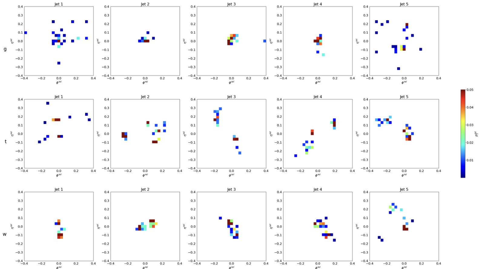
Jet data can also be represented as images. The following examples were produced using the synthetically simulated JetNet dataset. The question is then whether the patterns inside these images can help us infer which particle produced a particular jet.

A small guide to the names¶

First you should pardon poor physicists for not coming up with better names, nonetheless the following might help the curious souls. The feature names contain several pieces of information. For example,

d2_a1_b2_mmdt

can be read as

D2 observable | α = 1 | β = 2 | measured after mMDT grooming

Let us decode the notation carefully.

• zlogz is slightly different from the other variables. It describes how the jet momentum is shared among its constituent particles.

• C1, C2, D2, M2, and N2 are the names of different families of jet-substructure observables. The letters label different mathematical combinations of energy-correlation functions; they are not independent physical parameters.

• The number in C1, C2, D2, M2, or N2 indicates the level of internal structure being examined. In this dataset, C1 mainly describes one-prong properties such as the overall spread of a jet, while the observables ending in 2 are mainly designed to distinguish one-prong jets from jets with two hard branches.

• b0, b1, and b2 mean that the angular exponent (\beta) is set to

  $$\beta=0,\qquad \beta=1,\qquad \beta=2,$$

  (1)

  respectively.

  The energy-correlation functions contain angular factors schematically of the form

  $$\theta_{ij}^{\beta},$$

  (2)

  where $\theta_{ij}$ measures the angular separation between particles $i$ and $j$.

  Therefore:

  • $\beta=0$: the angular separation receives no additional weighting;

  • $\beta=1$: the observable depends linearly on the angle;

  • $\beta=2$: particles separated by larger angles receive relatively more weight.

• a1 means that a second angular exponent, written as $\alpha$, has been fixed to

  $$\alpha=1.$$

  (3)

  This appears in a generalized version of the $D_2$ observable in which the two-particle and three-particle correlations are allowed to use different angular exponents.

• mmdt means that the observable was measured after applying the modified Mass Drop Tagger. This grooming procedure removes soft, wide-angle radiation so that the harder internal structure of the jet becomes easier to study.

For example:

There is also a small curiosity in this dataset:

d2_b1_mmdt
d2_a1_b1_mmdt

represent the same choice $\alpha=\beta=1$, so their numerical values are identical in this particular dataset.

The main physical idea remains simple: changing $\alpha$ and $\beta$ changes how strongly an observable responds to the angular pattern of radiation inside the jet. The dataset therefore gives the neural network several different views of the same jet.

Let us now look briefly at what is hiding behind these names, for the first reading you can ignore the following details and may come back later to this page to learn them at your own time and pace.

The zlogz observable¶

Suppose that constituent $i$ carries a fraction $z_i$ of the total jet momentum:

These momentum fractions satisfy

The zlogz feature is

Because $0\leq z_i\leq 1$, we have $\log z_i\leq 0$, and therefore zlogz is normally negative.

This is closely related to the Shannon entropy,

Therefore,

This gives it a simple interpretation:

• if one particle carries nearly all the jet momentum, zlogz is closer to zero;

• if the momentum is shared among many particles, zlogz becomes more negative;

• equivalently, the corresponding Shannon entropy becomes larger.

For example, if the momentum is shared equally among $N$ particles,

then

Thus, zlogz measures how concentrated or distributed the momentum flow is inside the jet.

Two-particle and three-particle energy correlations¶

Let $z_i$ be the momentum fraction of particle $i$, and let $\theta_{ij}$ represent the angular separation between particles $i$ and $j$.

A two-particle energy correlation has the schematic form

It examines pairs of particles and asks how much momentum they carry and how far apart they are.

A three-particle energy correlation has the schematic form

It examines groups of three particles and is sensitive to more complicated internal structures.

The $C_1$, $C_2$, and $D_2$ observables¶

Ignoring some normalization conventions, the observables are constructed schematically as

and

These ratios compare the amount of three-particle structure with the amount of two-particle structure.

The $D_2$ observable is particularly useful for distinguishing:

• a jet with one dominant core, such as many ordinary quark or gluon jets;

• a jet with two hard internal branches, such as a boosted $W$ or $Z$ jet.

Why do some $D_2$ observables contain both $\alpha$ and $\beta$?¶

The generalized version allows the three-particle and two-particle correlations to use different angular exponents:

Therefore,

d2_a1_b2_mmdt

corresponds to

The numerator and denominator are then looking at the angular pattern with different sensitivities.

When

the generalized expression reduces to the usual $D_2$ form. This explains why

d2_b1_mmdt

and

d2_a1_b1_mmdt

contain the same information.

The $M_2$ and $N_2$ observables¶

The $M_2$ and $N_2$ observables are constructed using generalized energy-correlation functions.

They are written schematically as

and

The symbols ${}_1e_n$ and ${}_2e_n$ represent slightly different ways of combining the angular separations among groups of particles.

The detailed definitions are not important for our neural-network exercise. The physical messages are:

• $M_2$ was designed to identify two-prong structure particularly well after jet grooming;

• $N_2$ also identifies two-prong structure but does not require us to first choose explicit subjet axes;

• both provide alternative views of the same internal radiation pattern.

The main lesson is that these complicated-looking feature names encode three fairly simple ingredients:

1. which type of particle correlation is being measured;

2. how strongly angular separation is weighted;

3. whether soft radiation was removed before calculating the observable.

The equations may look formidable, but physically they are different ways of asking:

How is the energy arranged inside this jet?

❓ Exercise¶

Q23: What happens if classes overlap significantly? How does that affect the theoretical maximum accuracy our model can achieve?

Q24: Why do we normalize features using StandardScaler? What would happen to the weights in the first layer if one feature ranged from 0 to 1 and another ranged from 0 to 1,000,000? (Hint: Think about gradients and learning rates).

Q25: Examine the class distributions. Are they balanced or unbalanced? How does class imbalance affect evaluation metrics (e.g., standard accuracy vs balanced accuracy)?

Define the Model Architecture¶

Here we define our custom neural network class by inheriting from nn.Module. In PyTorch, we define our layers in __init__ and the network’s forward logic in forward.

❓ Exercise¶

Q26: Parameter Scaling: Change hidden_dim from 32 to 8, 64, 128, and 256. Note down how the parameter count changes. Can you compute the formula for the number of parameters in this model? (Hint: don’t forget biases!)

Linear(input_dim → hidden_dim)
Linear(hidden_dim → num_classes)

the first layer contains

$$
(\text{input\_dim}\times\text{hidden\_dim})+\text{hidden\_dim}
$$

parameters, and the output layer contains

$$
(\text{hidden\_dim}\times\text{num\_classes})+\text{num\_classes}.
$$

Therefore,

$$
N_{\mathrm{parameters}}
=
(\text{input\_dim}+1)\,\text{hidden\_dim}
+
(\text{hidden\_dim}+1)\,\text{num\_classes}.
$$

For `input_dim = 16` and `num_classes = 5`,

$$
N_{\mathrm{parameters}}=22\,\text{hidden\_dim}+5.
$$

This gives:

- `hidden_dim = 8` $\rightarrow 181$ parameters
- `hidden_dim = 32` $\rightarrow 709$ parameters
- `hidden_dim = 64` $\rightarrow 1413$ parameters
- `hidden_dim = 128` $\rightarrow 2821$ parameters
- `hidden_dim = 256` $\rightarrow 5637$ parameters

Q27: Going Deeper (Coding Challenge): Modify the SimpleClassifier class (or write a new class DeepClassifier below) to add a second hidden layer. Your network flow should be:

• Linear(input_dim -> hidden_dim)

• ReLU()

• Linear(hidden_dim -> hidden_dim)

• ReLU()

• Linear(hidden_dim -> num_classes)

class DeepClassifier(nn.Module):
    def __init__(self, input_dim, hidden_dim, num_classes):
        super().__init__()

        self.layer1 = nn.Linear(input_dim, hidden_dim)
        self.layer2 = nn.Linear(hidden_dim, hidden_dim)
        self.output = nn.Linear(hidden_dim, num_classes)
        self.relu = nn.ReLU()

    def forward(self, x):
        x = self.relu(self.layer1(x))
        x = self.relu(self.layer2(x))
        return self.output(x)


model = DeepClassifier(
    input_dim=train_X.shape[1],
    hidden_dim=64,
    num_classes=len(class_names),
)

Q28: Dropout Regularization (Coding Challenge): Insert a dropout layer (nn.Dropout(p=0.3)) after the activation function(s) to mitigate overfitting. What does dropout do during training, and how does it behave during evaluation (model.eval())?

class DeepClassifierWithDropout(nn.Module):
    def __init__(self, input_dim, hidden_dim, num_classes):
        super().__init__()

        self.layer1 = nn.Linear(input_dim, hidden_dim)
        self.layer2 = nn.Linear(hidden_dim, hidden_dim)
        self.output = nn.Linear(hidden_dim, num_classes)

        self.relu = nn.ReLU()
        self.dropout = nn.Dropout(p=0.3)

    def forward(self, x):
        x = self.dropout(self.relu(self.layer1(x)))
        x = self.dropout(self.relu(self.layer2(x)))
        return self.output(x)

DataLoader, Optimizer, and Loss¶

Next, we prepare our DataLoader for training, and choose our loss function and optimizer. These three components dictate how batches are loaded, how errors are quantified, and how weights are adjusted.

❓ Exercise¶

Q29: Batch Size Sweep: What happens if you change batch_size to 8, 16, 64, or 128? How does batch size affect training speed (seconds per epoch) and the smoothness of the loss curve?

Q30: Optimizer Experimentation: Replace Adam with standard stochastic gradient descent (torch.optim.SGD(model.parameters(), lr=0.01)). Does standard SGD learn faster or slower than Adam? Why does Adam converge faster in complex settings?

Q31: L2 Regularization: Add weight_decay=1e-4 to the Adam optimizer. Try values of 0, 1e-5, 1e-3, and 1e-2. How does L2 weight decay combat overfitting?

The Training Loop¶

The heart of deep learning in PyTorch is the training loop. We iterate over our epochs and mini-batches, performing forward passes, gradient calculations, and optimizer steps.

❓ Exercise¶

Q32: Underfitting vs. Overfitting: Run the training for 5, 20, and 100 epochs. At what point does the training loss stop decreasing significantly? Does the model begin to overfit if trained for too long?

Q33: Early Stopping Coding Challenge: Modify the training loop below (or implement a new version) to incorporate Early Stopping.

• Instruction: Evaluate validation loss at the end of each epoch. Keep track of the best validation loss. If the validation loss does not improve for 5 consecutive epochs, print a message and break the loop early.

import copy
from torch.utils.data import random_split

# Split the existing training tensors into a smaller training set
# and a validation set.
full_training_dataset = TensorDataset(train_X, train_Y)

n_validation = int(0.2 * len(full_training_dataset))
n_training = len(full_training_dataset) - n_validation

training_subset, validation_subset = random_split(
    full_training_dataset,
    [n_training, n_validation],
    generator=torch.Generator().manual_seed(42),
)

early_train_loader = DataLoader(
    training_subset,
    batch_size=32,
    shuffle=True,
)

validation_loader = DataLoader(
    validation_subset,
    batch_size=256,
    shuffle=False,
)

patience = 5
best_validation_loss = float("inf")
epochs_without_improvement = 0
best_state = None

for epoch in range(100):
    model.train()

    for batch_X, batch_Y in early_train_loader:
        batch_X = batch_X.to(device)
        batch_Y = batch_Y.to(device)

        optimizer.zero_grad()
        logits = model(batch_X)
        loss = criterion(logits, batch_Y)
        loss.backward()
        optimizer.step()

    model.eval()
    validation_loss = 0.0

    with torch.no_grad():
        for batch_X, batch_Y in validation_loader:
            batch_X = batch_X.to(device)
            batch_Y = batch_Y.to(device)

            logits = model(batch_X)
            validation_loss += criterion(logits, batch_Y).item()

    validation_loss /= len(validation_loader)

    print(
        f"Epoch {epoch + 1:03d} | "
        f"validation loss = {validation_loss:.4f}"
    )

    if validation_loss < best_validation_loss - 1e-5:
        best_validation_loss = validation_loss
        best_state = copy.deepcopy(model.state_dict())
        epochs_without_improvement = 0
    else:
        epochs_without_improvement += 1

    if epochs_without_improvement >= patience:
        print("Early stopping: validation loss stopped improving.")
        break

# Restore the best validation model.
if best_state is not None:
    model.load_state_dict(best_state)

Evaluate the Model¶

We must test our model on unseen data, Since thats the final goal anyway. During evaluation, we put the model in .eval() mode and wrap our code in with torch.no_grad(): to turn off gradient computation (saving memory and compute).

❓ Exercise¶

Q34: Inspect Predictions (Coding challenge): Write a quick snippet to print the first 10 predictions alongside their true labels. Identify which predictions are correct and which are wrong.

preds_cpu = preds.detach().cpu()
truth_cpu = test_Y.detach().cpu()

for i in range(10):
    predicted_class = class_names[preds_cpu[i].item()]
    true_class = class_names[truth_cpu[i].item()]
    status = "correct" if predicted_class == true_class else "wrong"

    print(
        f"Sample {i:02d}: "
        f"predicted = {predicted_class}, "
        f"true = {true_class}, "
        f"result = {status}"
    )

Q35: Locate Misclassifications (Coding challenge): Print the index and feature values of 3 samples that the model predicted incorrectly. What might have confused the model?

preds_cpu = preds.detach().cpu()
truth_cpu = test_Y.detach().cpu()
test_X_cpu = test_X.detach().cpu()

wrong_indices = torch.where(preds_cpu != truth_cpu)[0]

# NOTE: Convert standardized features back to their original units.
original_test_features = scaler.inverse_transform(
    test_X_cpu.numpy()
)

for index in wrong_indices[:3]:
    i = index.item()

    print(f"\nTest index: {i}")
    print(
        "Predicted class:",
        class_names[preds_cpu[i].item()],
    )
    print(
        "True class:",
        class_names[truth_cpu[i].item()],
    )

    feature_values = pd.Series(
        original_test_features[i],
        index=feature_cols,
    )
    print(feature_values)

Q36: Confusion Matrix (Coding challenge): Use sklearn.metrics.confusion_matrix and matplotlib.pyplot to compute and plot a Confusion Matrix.

Which particle classes are most frequently confused with each other? For example, quark q vs gluon g, or W boson w vs Z boson z. Why does this make physical sense?

from sklearn.metrics import (
    confusion_matrix,
    ConfusionMatrixDisplay,
)

preds_cpu = preds.detach().cpu()
truth_cpu = test_Y.detach().cpu()

cm = confusion_matrix(
    truth_cpu.numpy(),
    preds_cpu.numpy(),
    labels=range(len(class_names)),
)

fig, ax = plt.subplots(figsize=(6, 6))

display = ConfusionMatrixDisplay(
    confusion_matrix=cm,
    display_labels=class_names,
)

display.plot(
    ax=ax,
    cmap="Blues",
    colorbar=False,
)

ax.set_title("Jet-classification confusion matrix")
plt.show()

Logits vs Softmax Probabilities¶

Our model outputs raw values called logits. To convert them into interpretable probabilities that sum to 1, we apply the Softmax activation.

❓ Exercise¶

Q37: Can you recognize something familiar from statistical mechanics in the cross-entropy loss?

Q38: CrossEntropyLoss Detail: Look back at Cell 4 where we defined our loss function as nn.CrossEntropyLoss(). Notice that our model’s last layer in Cell 3 is a nn.Linear layer that directly outputs raw logits, not probabilities. What should be passed from the model to nn.CrossEntropyLoss()?

Q39: Why does nn.CrossEntropyLoss NOT want us to add a Softmax layer at the end of our model?

What two operations are combined inside nn.CrossEntropyLoss?

Q40: What is the numerical stability benefit of combining Softmax and Log operations together instead of computing them separately? (Hint: Think about floating-point exponentiation overflow and underflow).

Save and Load the Model¶

Once you have trained your model, you’ll want to save its weights so you can deploy it later. In PyTorch, we save the state_dict() which contains the model’s weight and bias matrices.

❓ Exercise¶

Q41: Now it is time to put everything you have learned to the test.

Your objective is to modify the code across the cells, or write custom code in the scratch cell below, to achieve the highest possible test accuracy on the jet-classification dataset.

Explore some combination of the following:

1. Scale up the Data: Increase n_samples from 20000 to 50000, 150000, or use the entire 830,000 dataset.

2. Wider/Deeper Model: Add more layers and hidden units, for example layers of size 128 and 64.

3. Combat Overfitting: Introduce nn.Dropout(p=0.2) or nn.Dropout(p=0.4) and weight decay.

4. Learning Rate Scheduling: Start with a larger learning rate and reduce it as training progresses.

5. Batch Size Tuning: Try batch sizes such as 16, 32, 64, 128, and 256.

6. Optimizer Experimentation: Compare Adam, AdamW, RMSprop, or SGD with momentum.

Can you surpass 80% accuracy? Record your architecture, training strategy, and best test accuracy.

import copy

class ImprovedClassifier(nn.Module):
    def __init__(self, input_dim, num_classes):
        super().__init__()

        self.network = nn.Sequential(
            nn.Linear(input_dim, 128),
            nn.BatchNorm1d(128),
            nn.ReLU(),
            nn.Dropout(0.2),

            nn.Linear(128, 64),
            nn.BatchNorm1d(64),
            nn.ReLU(),
            nn.Dropout(0.2),

            nn.Linear(64, num_classes),
        )

    def forward(self, x):
        return self.network(x)


improved_model = ImprovedClassifier(
    input_dim=train_X.shape[1],
    num_classes=len(class_names),
).to(device)

improved_loader = DataLoader(
    TensorDataset(train_X, train_Y),
    batch_size=256,
    shuffle=True,
)

criterion = nn.CrossEntropyLoss()

optimizer = torch.optim.AdamW(
    improved_model.parameters(),
    lr=1e-3,
    weight_decay=1e-4,
)

scheduler = torch.optim.lr_scheduler.StepLR(
    optimizer,
    step_size=10,
    gamma=0.5,
)

for epoch in range(40):
    improved_model.train()

    running_loss = 0.0
    correct = 0
    total = 0

    for batch_X, batch_Y in improved_loader:
        batch_X = batch_X.to(device)
        batch_Y = batch_Y.to(device)

        optimizer.zero_grad()
        logits = improved_model(batch_X)
        loss = criterion(logits, batch_Y)
        loss.backward()
        optimizer.step()

        running_loss += loss.item()
        correct += (
            logits.argmax(dim=1) == batch_Y
        ).sum().item()
        total += len(batch_Y)

    scheduler.step()

    print(
        f"Epoch {epoch + 1:02d} | "
        f"loss = {running_loss / len(improved_loader):.4f} | "
        f"accuracy = {100 * correct / total:.2f}%"
    )

improved_model.eval()

with torch.no_grad():
    final_logits = improved_model(test_X.to(device))
    final_predictions = final_logits.argmax(dim=1)

    final_accuracy = (
        final_predictions == test_Y.to(device)
    ).float().mean().item()

print(f"Final test accuracy: {100 * final_accuracy:.2f}%")