Convolutional Neural Networks - A minicourse in ML for Physicist

Why Convolutional Neural Networks?¶

Images have structure. Nearby pixels are usually related, and the same pattern can appear in different parts of the image. For example, the curve of a handwritten digit may appear slightly shifted, but we still want the model to recognize it as the same digit.

This kind of repeated local structure is exactly what convolutional neural networks are designed to exploit.

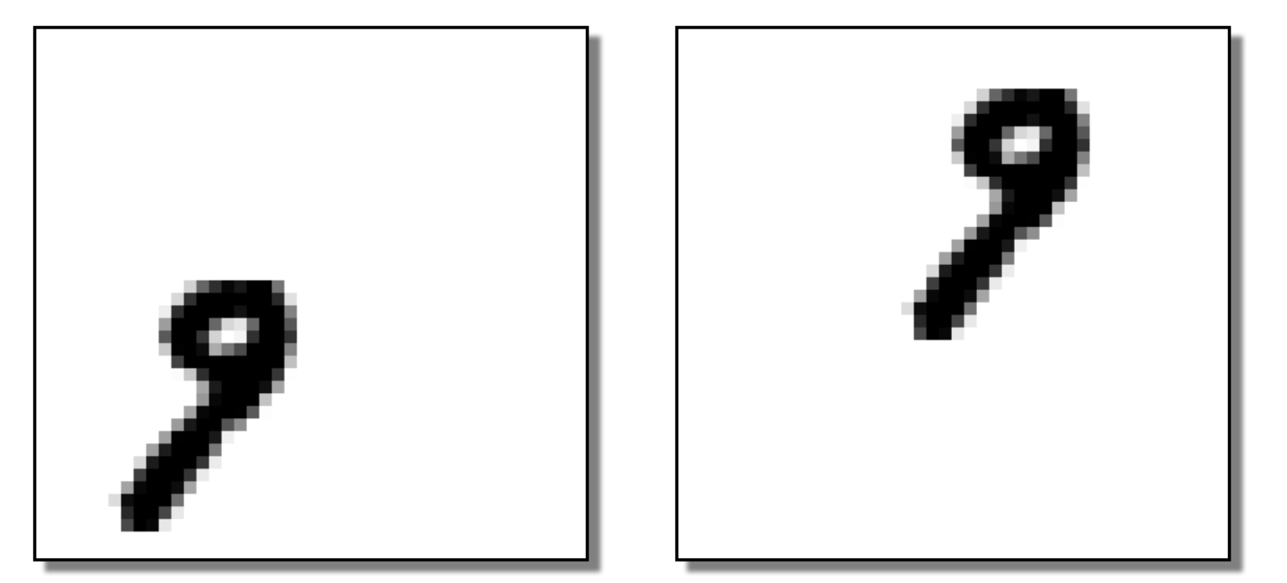
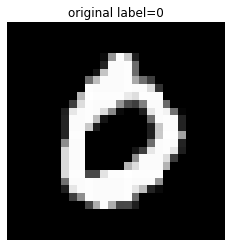
Figure 1:Two examples of the same digit from the MNIST dataset.

Convolution as a mathematical operation¶

A convolution combines two functions, say $f$ and $h$ , to produce a new function $g$ :

g(t)=(f*h)(t) = \int_{-\infty}^{\infty} f(\tau),h(t-\tau),d\tau.

(1)

Here, $h$ is often called the kernel. The kernel slides over the function $f$ and extracts local information.

For a two-dimensional image, the discrete version is

(f*h)[i,j] = \sum_m\sum_n f[m,n],h[i-m,j-n].

(2)

In image processing, $f[m,n]$ is the pixel value at position $(m,n)$ , and $h$ is a small matrix called a filter or kernel.

Convolutional Layer¶

In a convolutional layer, the convolution operation is performed as shown in the animation below. The filter slides over the input image, or over the feature maps from the previous layer, and extracts patterns such as edges, textures, and object parts.

During a forward pass, the filter scans the input according to its specifications, such as stride and padding.

stride tells us how many pixels the filter moves at each step. A stride of 1 means the filter moves one pixel at a time, while a stride of 2 skips every other position and produces a smaller output.
Padding means adding extra pixels, usually zeros, around the boundary of the image. This allows the filter to scan the edges properly and can help preserve the spatial size of the feature map.

At every filter position, a convolution-like operation is performed on the corresponding local patch of the input. This produces one output value in the next feature map.

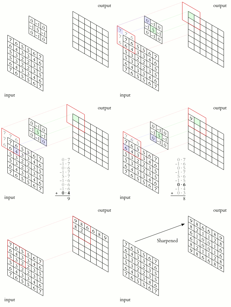
Figure 2:2D convolution animation. Image source: Wikimedia Commons.

Pooling Layer¶

A pooling layer is used in Convolutional Neural Networks to reduce the spatial dimensions of feature maps, namely their height and width, while preserving the most important information.

The pooling operation also uses a small window or kernel. This window moves across the input and extracts one representative value from each local region.

For example:

max pooling keeps the largest value in each local region;
average pooling keeps the average value in each local region.

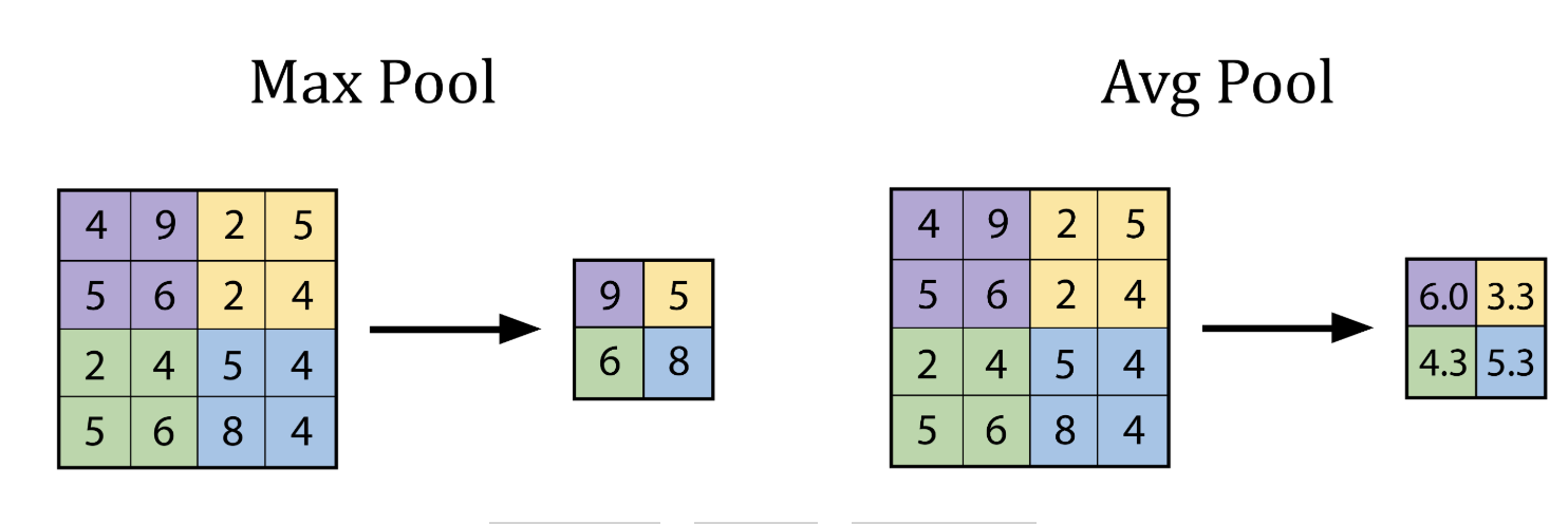
Figure 3:Illustration of a pooling operation.

The main advantages are:

it makes the model faster and lighter;
it can help reduce overfitting;
it helps the model focus on key features rather than exact pixel positions.

A useful visual explanation¶

One of the best visual explanations of CNNs is the excellent video by 3Blue1Brown.

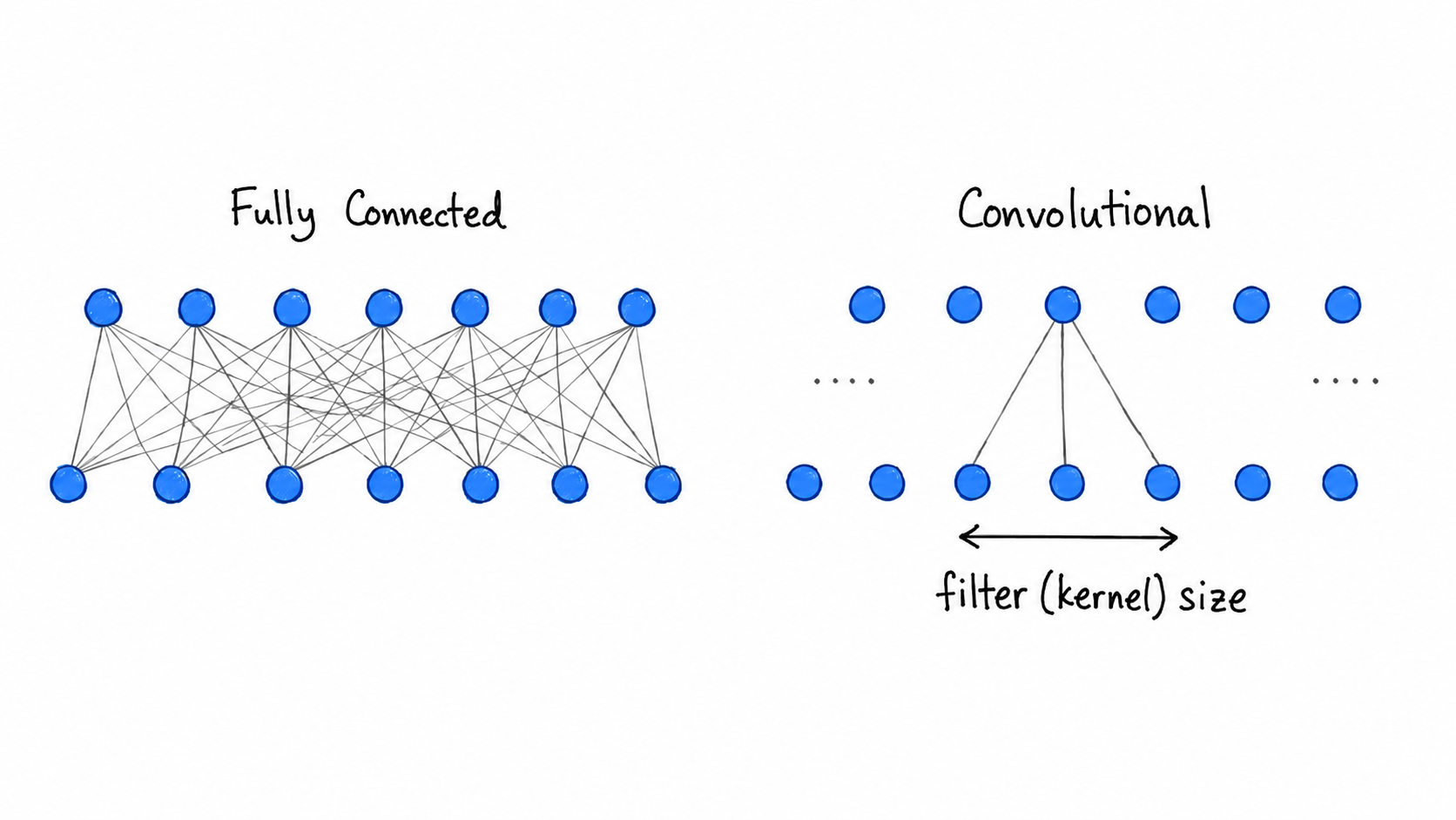
Figure 4:A visual comparison of convolutional operations.

Simple Example: 1D discrete Convolution¶

Let’s say you have a signal 𝑓 and a filter ℎ, the whole process of convolution can be summarised as the following for a given:

f = [3,2,1,0]

(3)

h=[1,0,-1]

(4)

Flip the filter

h_{flipped}=[-1,0,1]

(5)

Slide the filter across the input and multiply-and-sum at each step:

~~~~~~~~~~~~~~~~~~~~~~~~~~~~~~~[\fbox{3},2,1,0]

(6)

~~~~~~~~~~[-1,0,\fbox{1}]

(7)

$3*1=3$

~~~~~~~~~~~~~~~~~~~~~~~~~~~~~~~[\fbox{3},\fbox{2},1,0]

(8)

~~~~~~~~~~~~~~~~~~[-1,\fbox{0}, \fbox{1}]

(9)

$3*0 + 2*1 =2$

~~~~~~~~~~~~~~~~~~~~~~~~~~~~~~~[\fbox{3},\fbox{2},\fbox{1},0]

(10)

~~~~~~~~~~~~~~~~~~~~~~~~~~[\fbox{-1},\fbox{0},\fbox{1}]

(11)

$3*(-1) + 2*0 + 1*1 =-2$

~~~~~~~~~~~~~~~~~~~~~~~~~~~~~~~[3,\fbox{2},\fbox{1},\fbox{0}]

(12)

~~~~~~~~~~~~~~~~~~~~~~~~~~~~~~~~~[\fbox{-1},\fbox{0},\fbox{1}]

(13)

$2*(-1) + 1*0 + 0*1 =-2$

~~~~~~~~~~~~~~~~~~~~~~~~~~~~~~~[3,2,\fbox{1},\fbox{0}]

(14)

~~~~~~~~~~~~~~~~~~~~~~~~~~~~~~~~~~~~~~~~~[\fbox{-1},\fbox{0},1]

(15)

$1*(-1) + 0*0 =-1$

~~~~~~~~~~~~~~~~~~~~~~~~~~~~~~~[3,2,1,\fbox{0}]

(16)

~~~~~~~~~~~~~~~~~~~~~~~~~~~~~~~~~~~~~~~~~~~~~~~~~[\fbox{-1},0,1]

(17)

$0*(-1) =0$

Resulting convolved signal:

f*h= [3,2,-2,-2,-1,0]

(18)

Or this can be directly computed in python as

import numpy as np

a = np.convolve([3,2,1,0],(1,0,-1))

print(a)

[ 3  2 -2 -2 -1  0]

A physics analogy: Green’s functions¶

Convolution is also very natural in physics. Suppose we have a linear differential equation

\mathcal{L}\phi(x)=J(x),

(19)

where $\mathcal{L}$ is a linear differential operator, $\phi(x)$ is the field we want to solve for, and $J(x)$ is a source.

The Green’s function $G(x,x')$ is defined by

\mathcal{L}G(x,x')=\delta(x-x').

(20)

Once we know the Green’s function, the solution is

\phi(x) = \int dx',G(x,x')J(x').

(21)

So the field at $x$ is built by summing the influence of the source $J(x')$ at all other points, weighted by the Green’s function.

For example, for a scalar field,

(\Box + m^2)\phi(x)=J(x),

(22)

the Green’s function satisfies

(\Box + m^2)G(x,x')=\delta(x-x').

(23)

In quantum field theory, this Green’s function is closely related to the propagator. In momentum space, one can derive the free scalar propagator as

G(p) = \frac{i}{p^2-m^2+i\epsilon}.

(24)

Key takeaway: CNN kernels and Green’s functions

A useful physics way to think about CNNs is:

\boxed{ \text{CNN kernel} \quad \sim \quad \text{discrete, learnable Green's function} }

(25)

In physics, a Green’s function tells us how a source at one point contributes to a field elsewhere:

\phi(x) = \int dx'\,G(x,x')J(x').

(26)

In a CNN, a convolutional kernel tells us how nearby pixels contribute to a feature value:

y[a,b] = \sum_i\sum_j K[i,j]\,x[a-i,b-j].

(27)

So both objects describe how information from nearby or source points is combined to produce a response.

The difference is that a Green’s function is usually fixed by a known differential operator, while a CNN kernel is learned from data.

CNN Implementation¶

Here we will use the MNIST database of large number of handwritten digits.

import torch
import torch.nn as nn
import torch.optim as optim
import torchvision
import torchvision.transforms as transforms
import torch.nn.functional as F
import matplotlib.pyplot as plt

# Set manual seed for reproducibility
torch.manual_seed(42)

# Loading the MNIST dataset, already included with torchvision dataset

transform = transforms.Compose([
    transforms.ToTensor()
])

train_set = torchvision.datasets.MNIST(root='./data', train=True, download=True, transform=transform)
train_loader = torch.utils.data.DataLoader(train_set, batch_size=64, shuffle=True)

test_set = torchvision.datasets.MNIST(root='./data', train=False, download=True, transform=transform)
test_loader = torch.utils.data.DataLoader(test_set, batch_size=1000, shuffle=False)

# Show a single image
def show_image(img, title=""):
    img = img.squeeze()
    plt.imshow(img, cmap='gray')
    plt.title(title)
    plt.axis('off')
    plt.show()

test_image, test_label = test_set[3]
show_image(test_image, title="original label={}".format(test_label))
print(test_image.shape)

torch.Size([1, 28, 28])

# Simple CNN model

class SimpleCNN(nn.Module):
    def __init__(self):
        super().__init__()

        # conv1: Input channels = 1 (grayscale), Output channels = 4, Kernel size = 3x3
        # Input image: 28x28 -> Output: (28 - 3 + 1) = 26x26
        self.conv1 = nn.Conv2d(in_channels=1, out_channels=4, kernel_size=3)

        # MaxPool1: 2x2 pooling reduces 26x26 to 13x13
        self.pool1 = nn.MaxPool2d(kernel_size=2, stride=2)

        # conv2: Input channels = 4, Output channels = 8, Kernel size = 3x3
        # Input: 13x13 -> Output: (13 - 3 + 1) = 11x11
        self.conv2 = nn.Conv2d(in_channels=4, out_channels=8, kernel_size=3)

        # MaxPool2: 2x2 pooling reduces 11x11 to 5x5
        self.pool2 = nn.MaxPool2d(kernel_size=2, stride=2)

        # Fully Connected (FC) Layer: Input = 8 feature maps * 5 * 5 = 200
        # Output = 10 classes (e.g., MNIST digits)
        self.fc = nn.Linear(in_features=8 * 5 * 5, out_features=10)

    def forward(self, x):
        x = self.pool1(F.relu(self.conv1(x)))  # Shape: [batch, 4, 13, 13]
        x = self.pool2(F.relu(self.conv2(x)))  # Shape: [batch, 8, 5, 5]
        x = x.view(-1, 8 * 5 * 5)              # Flatten to [batch, 200]
        x = self.fc(x)                         # Output: [batch, 10]
        return x

# Here goes the training
model = SimpleCNN()
criterion = nn.CrossEntropyLoss()
optimizer = optim.Adam(model.parameters(), lr=0.001)

print("Training the CNN...")
for epoch in range(10):  # few epochs for demonstration
    running_loss = 0.0
    for images, labels in train_loader:
        optimizer.zero_grad()
        outputs = model(images)
        loss = criterion(outputs, labels)
        loss.backward()
        optimizer.step()
        running_loss += loss.item()
    print(f"Epoch {epoch+1} - Loss: {running_loss:.3f}")

Training the CNN...
Epoch 1 - Loss: 420.520
Epoch 2 - Loss: 143.036
Epoch 3 - Loss: 112.597
Epoch 4 - Loss: 96.404
Epoch 5 - Loss: 86.154
Epoch 6 - Loss: 79.574
Epoch 7 - Loss: 73.306
Epoch 8 - Loss: 69.770
Epoch 9 - Loss: 66.393
Epoch 10 - Loss: 62.597

# Get one test image
test_image, test_label = test_set[0]
input_image = test_image.unsqueeze(0)  # add batch dim: [1, 1, 28, 28]

# Run through model
model.eval()
with torch.no_grad():
    x1 = torch.relu(model.conv1(input_image))
    x2 = model.pool1(x1)

    x3 = torch.relu(model.conv2(x2))
    x4 = model.pool2(x3)

    flat = x4.view(-1, 8 * 5 * 5)
    logits = model.fc(flat)
    probs = torch.softmax(logits, dim=1)
    prediction = probs.argmax(dim=1).item()

# Showing the original one

print(f"True Label: {test_label} | Predicted: {prediction}")
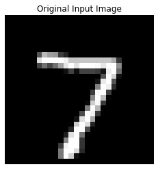
show_image(test_image, title="Original Input Image")

# Feature map visualisation

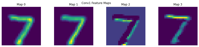
def show_feature_maps(tensor, title=""):
    tensor = tensor.squeeze()
    num_maps = tensor.shape[0]
    fig, axes = plt.subplots(1, num_maps, figsize=(15, 3))
    for i in range(num_maps):
        axes[i].imshow(tensor[i], cmap='viridis')
        axes[i].set_title(f"Map {i}")
        axes[i].axis('off')
    plt.suptitle(title)
    plt.show()

show_feature_maps(x1, "Conv1 Feature Maps")
show_feature_maps(x3, "Conv2 Feature Maps")

True Label: 7 | Predicted: 7


# Visualising the filter itself

def show_conv_filters(conv_layer, title=""):
    weights = conv_layer.weight.data.clone()
    num_filters = weights.shape[0]
    fig, axes = plt.subplots(1, num_filters, figsize=(12, 3))
    for i in range(num_filters):
        axes[i].imshow(weights[i, 0], cmap='gray')
        axes[i].set_title(f"Filter {i}")
        axes[i].axis('off')
    plt.suptitle(title)
    plt.show()

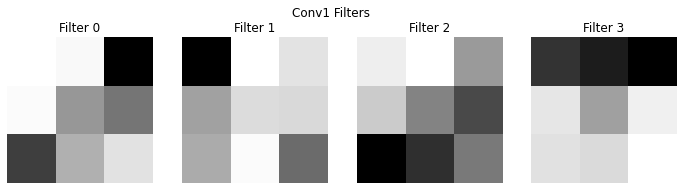
show_conv_filters(model.conv1, "Conv1 Filters")
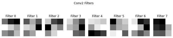
show_conv_filters(model.conv2, "Conv2 Filters")