The Imitation Game ¶ The imitation game or the Turing test refers to a test for assesing machine intelligence , proposed by the British mathematician and computer scientist Alan Turing in 1950.
The test is designed to asses a machine’s ability to exhibit intelligent behaviour equivalent to, or indistinguishable from that of a human.
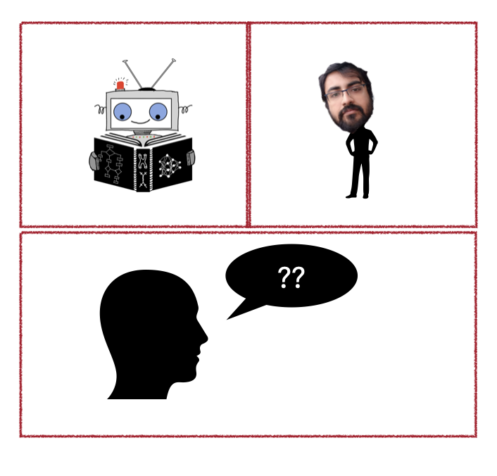
Figure 1: “Try this game with ChatGPT/DeepSeek”
Machine Learning: Quite crudely, machine learning can be thought of as a collection of tools and techniques that transforms data into decisions (hopefully good!!) by making some form of classification , like whether or not someone likes pineapple pizza, or some form of quantitavive predictions , like how long can someone run.
Machine Learning Classification ¶ One excellent example of classification is the classification tree itself. We will learn more about them soon.
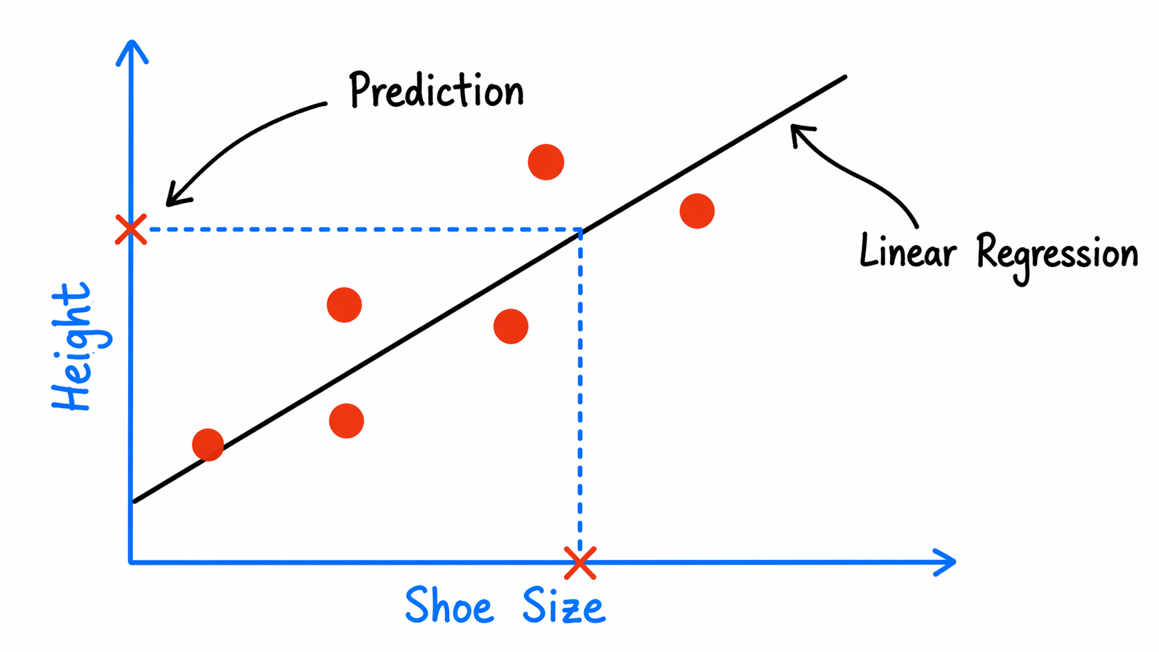
Machine Learning Regression ¶ Suppose we have a pile of Shoe-size vs Height data, and we want to make some predictions.
Figure 2: “Example: Linear Regression”
Different Types of ML ¶ Density estimation
Clustering maps
Dimensionality reduction
Outlier detection
Deep-Q learning
Self-driving car
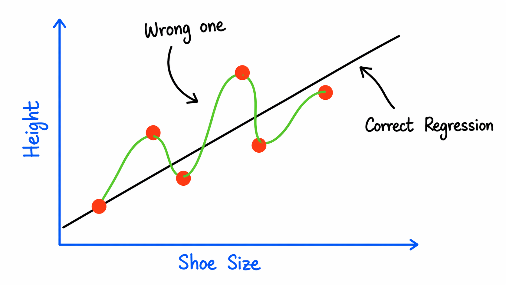
❓ Exercise ¶ Q7: How to stop the Green Squiggle from being the final answer??
Figure 3: “Wrong Regression”
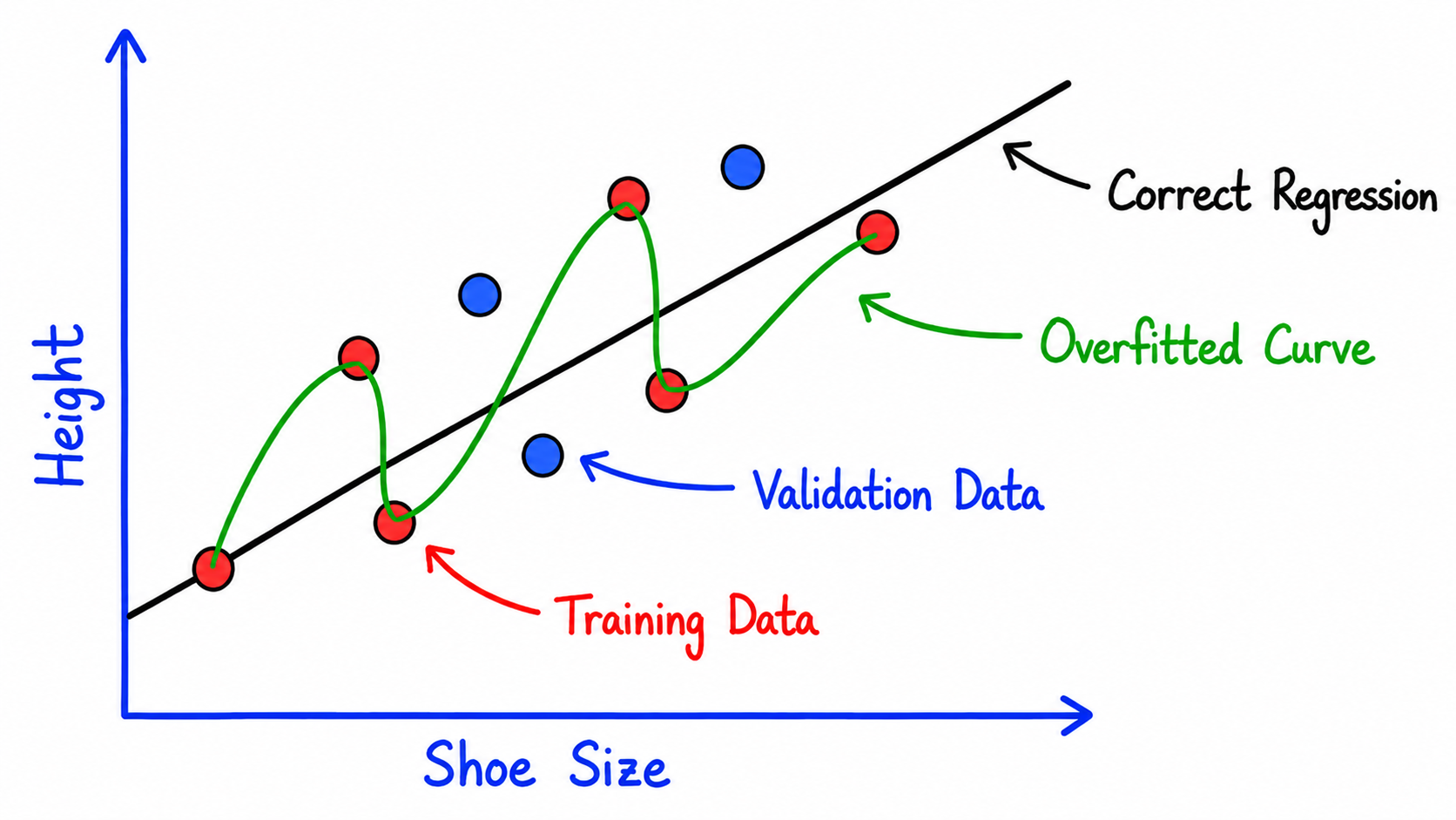
Answer: Add some validation point. If the green squiggle is the final answer then the prediction do will do worse for validation points.
Figure 4: “Correcting Regression”
There are tons of fancy machine learning methods and architectures available — like Deep Learning Convolutional Neural Networks and many others — and each month something new and exciting comes along. However, regardless of what we use, the most important question is how it performs on testing data , i.e., data that the model has not seen before .
Statistical Interlude: Data as Monte Carlo Samples ¶ In machine learning, we usually do not have access to the full probability distribution that generates the data.
Instead, we only see a finite dataset.
So a dataset should be thought of as a sample drawn from some underlying probability distribution.
Suppose the true data-generating distribution is
p ( ϕ ∣ source ) . p(\phi \mid \text{source}). p ( ϕ ∣ source ) . Here, ϕ \phi ϕ ϕ \phi ϕ
For simplicity, we often write
p ( ϕ ∣ source ) ≡ p ( ϕ ) . p(\phi \mid \text{source}) \equiv p(\phi). p ( ϕ ∣ source ) ≡ p ( ϕ ) . In many physics and machine learning problems, we assume that the training examples are independent and identically distributed , or i.i.d.
This means that each data point is drawn independently from the same probability distribution.
If we have N N N
{ ϕ 1 , ϕ 2 , … , ϕ N } , \{\phi_1,\phi_2,\ldots,\phi_N\}, { ϕ 1 , ϕ 2 , … , ϕ N } , then the i.i.d. assumption means
p ( ϕ 1 , ϕ 2 , … , ϕ N ) = ∏ i = 1 N p ( ϕ i ) . p(\phi_1,\phi_2,\ldots,\phi_N)
=
\prod_{i=1}^{N}p(\phi_i). p ( ϕ 1 , ϕ 2 , … , ϕ N ) = i = 1 ∏ N p ( ϕ i ) . This is an extremely useful assumption. It says that every event is generated by the same physical/statistical rule, but each event is still a fresh random draw. In collider physics, this is a very natural way to think.
Each collision event is random, but it is not arbitrary. It is sampled from a probability distribution determined by the underlying physics, detector response, reconstruction procedure, and event selection.
Loosely, in everyday machine learning it may feel awkward to imagine that all cat images, all books, or all possible text sequences are random samples from some enormous probability distribution. This is especially true when thinking about large language models.
But in physics, this viewpoint is much more natural. Every possible collision event is expected to follow some probability distribution dictated by the Standard Model, or by physics beyond the Standard Model.
So for collider physics, the statement
data ∼ p ( ϕ ) \text{data} \sim p(\phi) data ∼ p ( ϕ ) is not just a mathematical convenience. It is very close to how we believe nature produces events.
Now suppose we want to compute the average value of some observable f ( ϕ ) f(\phi) f ( ϕ )
⟨ f ( ϕ ) ⟩ p = ∫ d ϕ p ( ϕ ) f ( ϕ ) . \langle f(\phi)\rangle_p
=
\int d\phi \, p(\phi) f(\phi). ⟨ f ( ϕ ) ⟩ p = ∫ d ϕ p ( ϕ ) f ( ϕ ) . But in real life, we do not know the full distribution p ( ϕ ) p(\phi) p ( ϕ )
p ( ϕ ) ≈ 1 N ∑ i = 1 N δ ( ϕ − ϕ i ) . p(\phi)
\approx
\frac{1}{N}\sum_{i=1}^{N}\delta(\phi-\phi_i). p ( ϕ ) ≈ N 1 i = 1 ∑ N δ ( ϕ − ϕ i ) . Substituting this into the expectation value gives
⟨ f ( ϕ ) ⟩ p = ∫ d ϕ p ( ϕ ) f ( ϕ ) ≈ ∫ d ϕ [ 1 N ∑ i = 1 N δ ( ϕ − ϕ i ) ] f ( ϕ ) . \langle f(\phi)\rangle_p
=
\int d\phi \, p(\phi) f(\phi)
\approx
\int d\phi
\left[
\frac{1}{N}\sum_{i=1}^{N}\delta(\phi-\phi_i)
\right]
f(\phi). ⟨ f ( ϕ ) ⟩ p = ∫ d ϕ p ( ϕ ) f ( ϕ ) ≈ ∫ d ϕ [ N 1 i = 1 ∑ N δ ( ϕ − ϕ i ) ] f ( ϕ ) . Using the property of the delta function,
∫ d ϕ δ ( ϕ − ϕ i ) f ( ϕ ) = f ( ϕ i ) , \int d\phi \, \delta(\phi-\phi_i)f(\phi)=f(\phi_i), ∫ d ϕ δ ( ϕ − ϕ i ) f ( ϕ ) = f ( ϕ i ) , we get
⟨ f ( ϕ ) ⟩ p ≈ 1 N ∑ i = 1 N f ( ϕ i ) . \langle f(\phi)\rangle_p
\approx
\frac{1}{N}\sum_{i=1}^{N}f(\phi_i). ⟨ f ( ϕ ) ⟩ p ≈ N 1 i = 1 ∑ N f ( ϕ i ) . A training dataset is a Monte Carlo approximation to the true data-generating distribution.
So whenever we compute an average over the dataset, we are really estimating an expectation value:
true average ≈ sample average . \text{true average}
\approx
\text{sample average}. true average ≈ sample average . In other words,
⟨ f ( ϕ ) ⟩ p ≈ 1 N ∑ i = 1 N f ( ϕ i ) \boxed{
\langle f(\phi)\rangle_p
\approx
\frac{1}{N}\sum_{i=1}^{N}f(\phi_i)
} ⟨ f ( ϕ ) ⟩ p ≈ N 1 i = 1 ∑ N f ( ϕ i ) This is the statistical heart of why more data usually helps.
The Monte Carlo estimation error typically decreases like
1 N . \frac{1}{\sqrt{N}}. N 1 . So if we increase the dataset size, the empirical average becomes a better approximation to the true expectation value.
However, the improvement is slow. To reduce the statistical error by a factor of 10, we usually need about 100 times more data.
A few words on Monte Carlo ¶ Monte Carlo methods use randomness to estimate quantities that may be difficult to compute exactly. In this sense, a dataset is already doing something Monte Carlo-like: it gives us random samples from an unknown distribution, and we use these samples to estimate averages, probabilities, losses, and other quantities.
The name Monte Carlo comes from the famous casino district in Monaco.
The idea is that these methods rely on randomness, chance, and repeated sampling, much like gambling games in a casino. Historically, the name became associated with random-sampling methods developed in the context of nuclear physics calculations.
Machine learning training data are not the full truth.
They are finite samples from an underlying distribution.
Therefore, training a model is not just fitting points. It is an attempt to learn stable statistical structure from noisy Monte Carlo samples.